Mixture Models

import numpy as np
import matplotlib.pyplot as plt
import seaborn as sns
from scipy import stats
from matplotlib import cm

sns.set_theme()

In mixture models we assume that the input examples come from different potentially unobserved types (groups, clusters etc.). We assume that there are $m$ underlying types where each type $z$ occurs with a certain probability $ \mathbb{P}(z) $. The examples of the type $z$ are then conditionally distributed $ \mathbb{P}(\mathbf{x}|z ) $. The observations $ \mathbf{x} $ then come from a so called mixture distribution, which is just the weighted sum of the type probability times the conditional type probability

A mixture of gaussians model has the form

Data generation

During the data generation, with probability $ \mathbb{P}(z) $ class $z_j$ is chosen and the sample points $ \mathbf{x} $ are chosen from the conditional distribution $ \mathbb{P}(\mathbf{x} | z = j ) $. For a two class system, our sample points $ \mathbf{x} $ could then have been generated in two ways. We thus would like to find out the underlying distribution of our observations.

Latent Variable Models (LVM).

In the model $ \mathbb{P}(\mathbf{x} | z=j, \mathbf{\theta})$ the class indicator variable $z$ is latent. This means that $z$ is a variable that can only be indirectly inferred through mathematical models from other observable variables that can directly be observed. They are not directly measurable / observed. This then is an example of a large class of latent variable models (LVM). We use the Bayesian network (DAG) as a graphical representation of the join distribution of RVs as $\mathbb{P}(x_1, …, x_n) = \prod_{i=1}^n \mathbb{P}(x_i | parents(x_i))$, i.e.

In this graph our RVs are $ \mathbf{x}_i$ and $z_i$ which hold the parameters $ \mathbf{\mu}, \Sigma $ and $\mathbf{\pi}$.

If we now assume we have a two component mixture model then we can write our probability of $ \mathbf{x}$ given the parameters $ \mathbf{\theta} $ as followed

Mixture density estimation

If we knew our generating component $z_i$, the estimation of the points $ \mathbf{x} $ would be easy. Let $\delta(j|i)$ be an indicator function of whether an example $i$ is labeled $j$. Then for our class distribution we can estimate the parameters by

Even though we don’t know our labels, we can estimate them based on our calculated distributions.

Our soft labels i.e. the prob of a given latent variable is then just the posterior. Thus by calculating the posterior we get the mixture probability. We write our soft labels as $ \hat{p}(j|i) $, thus the probability of point $i$ being of class $j$. $z_i$ here is then the class of $ \mathbf{x}_i $.

EM-Algorithm

• E-Step: Softly assign examples to mixture models

• M-Step: Estimate new mixture parameters $ \mathbf{\theta}^{t+1}$ based on soft assignements

Bayesian model selection

Because we do not know the amount of mixture components there are in our data, we have to perform a model seletion. A simple way to approximate the amount of mixture components is to find $m$ that minimizes the overall description length of the model, i.e. the BIC for example.

where $n$ is the number of training points, $\hat{\mathbf{\theta}}_m$ are the maximum likelihood parameters of the $m$-mixture component model and $d_m$ is the number of parameters in the $m$-mixture component model.

Convergence of the EM-Algorithm

Because the EM-algorithm monotonically increases the log-likelihood of the training data, the EM-algorithm is guaranteed to converge atleast to a local optima

with

For repetition the EM-Algorithm looks like

• Step 0: Initialise parameter setting $ \mathbf{\theta} = \mathbf{\theta}^0$

• E-Step: Softly assign examples to mixture models

• M-Step: find the new setting of the parameter $ \mathbf{\theta}^{t+1} $ by maximizing the log-likelihood of the inferred (or expected complete) data

The expected complete log-likelihood $Q(\mathbf{\theta}, \mathbf{\theta}^t)$ is called the auxiliary objective. The auxiliary function gives us new parameters which maximizes the expected log likelihood. This is the expectation of the log-likelihood with respect to the probability of the class assignements given the current model and input $ \mathbf{x} $.

Jensen’s inequality

For a convex function there exist always a secant line above the graph between two points

x = np.arange(-2, 2, 0.01)
y = x**2

line = 1.25 * x + 1

plt.title('Jensens Inequality')
plt.plot(x, y, label='function')
plt.plot(x, line, label='Upper bound')
plt.legend()
plt.show()

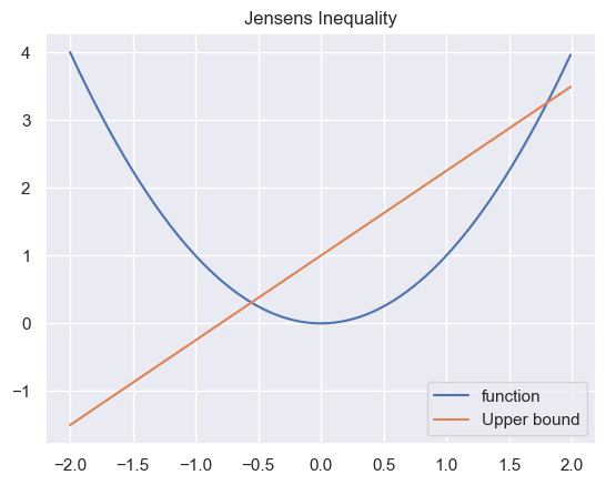
Thus for $a\in[0, 1]$ we get our line $af(x_1) + (1 - a)f(x_2)$ which gives us then the jensen’s inequality

For then X which is a RV and $\phi$ a convex function, we get

now if then $\phi$ is convex, $\psi = - \phi$ is a concave function and we get

for example the logarithm, which is a concave function which yields $\log (\mathbb{E}[X]) \geq \mathbb{E}[\log(X)]$.

Gibbs inequality

Note that the KL-divergence is a non-negative value and iff $q=p \Rightarrow \mathbb{KL} = 0$, else $\mathbb{KL} \neq 0$.

Convergence proof

Looking at the log-likelihood of our EM, we assume the latent variables are distributed according to $ q(z_i) $. We don’t make any assumptions regarding $ q(z_i) $, other than that it is a valid probability distribution. \(\begin{align*} I(\mathbf{\theta}) &= \sum_{i=1}^n \log \mathbb{P}(\mathbf{x}_i | \mathbf{\theta}) \\ &= \sum_{i=1}^n \log \sum_{z_i} \mathbb{P}(\mathbf{x}_i, z_i | \mathbf{\theta}) \\ &= \sum_{i=1}^n \log \sum_{z_i} q(z_i) \frac{\mathbb{P}(\mathbf{x}_i, z_i | \mathbf{\theta})}{q(z_i)} \\ &= \sum_{i=1}^n \log \mathbb{E}_{q_i} \frac{\mathbb{P}(\mathbf{x}_i, z_i | \mathbf{\theta})}{q(z_i)} \\ &\geq \sum_{i=1}^n \sum_{z_i} q(z_i) \log \frac{\mathbb{P}(\mathbf{x}_i, z_i | \mathbf{\theta})}{q(z_i)} \\ & =: Q(\theta, q) \end{align*}\)

Thus we get a lower bound on our likelihood which is valid for any given postive distribution q. We then would like to pick $q$ which gives the tighest lower bound, i.e. the one that maximizes the auxilirary function. This is the E-step of the EM algorithm. At time $t$, we assume we have chosen $q^t$ based on current parameters $ \mathbf{\theta}^t $. In the M-Step wou would then like to maximize the expected complete log-likelihood

This new $ \mathbf{\theta}$ maximizes our lower bound at step $t$. Thus the $ \mathbf{\theta} $ which we want to maximize in the M-Step also maximizes our lower bound, because our choise of $q^t$ depends on $ \mathbf{\theta}^t $.

The second expression is what we want to do in the M-Step, i.e. we would like to maximize our Expected complete log likelihood which signifies the likelihood (probability) of our assignements of the points being of the correct class. The equility follows from

Because the second term is independent of $ \mathbf{\theta}^t $, if we want to maximize the expected complete log likelihood, we maximize our lower bound.

For now the lower bound we rewrite this as

with

Thus the lower bound always touches a specific point of the log-likelihood. We then maximize our auxilirary function and move in that direction, still touching the true log-likelihood. This causes us to monotonically increase our log-likelihood which converges then to a local optima of the true log-likelihood. The monotonic increase thus comes from

We can thus summarize the EM-algorithm as

1. E-Step: $\mathbf{q}^t = \arg \max_{\mathbf{q}} Q(\mathbf{\theta}^t, \mathbf{q})$
2. M-Step: $ \mathbf{\theta}^{t+1} = \arg \max_{\mathbf{\theta}} Q(\mathbf{\theta}, \mathbf{\theta}^t)$

In the E-Step we estimate the expected value for each latent variable, i.e. the soft labels and in the M-Step we optimize the parameters with these new soft labels.

def EM(X: np.array, K: int) -> tuple[np.array, np.array]:
    means = np.array([[-1, -1], [1, 1]])
    covs = np.array([[[1, 0.8], [0.8, 1]], [[1, -0.4], [-0.4, 1]]])
    
    pz = np.zeros(K) + (1 / K)
    
    iteration = 0
    converged = False
    while not converged:
        for k in range(K):
            
            # E-Step
            nominator = pz[k] * stats.multivariate_normal(mean=means[k], cov=covs[k]).pdf(X) + 1e-4
            denominator = np.sum([pz[i] * stats.multivariate_normal(mean=means[i], cov=covs[i]).pdf(X) + 1e-4 for i in range(K)])
            r = nominator / denominator
            pz[k] = np.mean(r)
            # M-Step
            means[k] = np.sum([r[i] * X[i] for i in range(len(X))]) / np.sum(r)
            
            cov = np.zeros((2, 2))
            
            for i in range(len(X)):
                cov += r[i] * np.outer(X[i] - means[k], X[i] - means[k])
            covs[k] = cov /  np.sum(r)  
            
            #means[k] = r.T @ X / np.sum(r) + 1e-4
            
            #covs[k] = ((X * r[:, None])  - means[k]).T @ (X - means[k]) / np.sum(r)  + 1e-4 
            
            
            log_likelihood = ...
            
        iteration += 1
        
        if iteration > 100:
            print('stop')
            break
    return means, covs

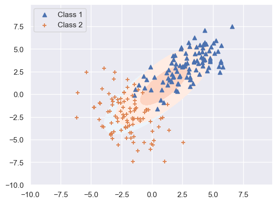
np.random.seed(0)
x = np.arange(-10, 10, 0.1)
X, Y = np.meshgrid(x, x)
pos = np.dstack((X, Y))

norm1 = stats.multivariate_normal([3, 3], [[3, 2], [2, 3]])
norm2 = stats.multivariate_normal([-2, -2], [[2, 1], [-2, 5]])

class1 = norm1.rvs(size=100)
class2 = norm2.rvs(size=100)

data = np.vstack((class1, class2))
mean , cov = EM(data, 2)
print(mean, cov)
x = np.arange(-10, 10, 0.1)

norm1_pred = stats.multivariate_normal(mean[0], cov[0])
norm2_pred = stats.multivariate_normal(mean[1], cov[1])

Z1 = norm1_pred.pdf(pos)
Z2 = norm2_pred.pdf(pos)

levels = np.arange(0.0, 0.1, 0.01) + 0.01

plt.contourf(X, Y, Z1, levels, extent=(-3,3,-2,2),cmap=cm.Blues, alpha=1)
plt.contourf(X, Y, Z2, levels, extent=(-3,3,-2,2),cmap=cm.Reds, alpha=1)
plt.scatter(class1[:, 0], class1[:, 1], marker='^', label='Class 1')
plt.scatter(class2[:, 0], class2[:, 1], marker='+', label='Class 2')
plt.legend()
plt.show()

stop
[[0 0]
 [1 1]] [[[ 8.40027867  6.95616178]
  [ 6.95616178 10.5413611 ]]

 [[ 8.52422479  7.14547898]
  [ 7.14547898 10.74023968]]]

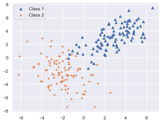
np.random.seed(0)
x = np.arange(-10, 10, 0.1)
X, Y = np.meshgrid(x, x)
pos = np.dstack((X, Y))


norm1 = stats.multivariate_normal([3, 3], [[3, 2], [2, 3]])
norm2 = stats.multivariate_normal([-2, -2], [[2, 1], [-2, 5]])

class1 = norm1.rvs(size=100)
class2 = norm2.rvs(size=100)

Z1 = norm1.pdf(pos)
Z2 = norm2.pdf(pos)

levels = np.arange(0.0, 0.1, 0.01) + 0.01

#plt.contourf(X, Y, Z1, levels, extent=(-3,3,-2,2),cmap=cm.Blues, alpha=1)
#plt.contourf(X, Y, Z2, levels, extent=(-3,3,-2,2),cmap=cm.Reds, alpha=1)
plt.scatter(class1[:, 0], class1[:, 1], marker='^', label='Class 1')
plt.scatter(class2[:, 0], class2[:, 1], marker='+', label='Class 2')
plt.legend()
plt.show()

Conditional Mixtures

Sometimes a regression or classification problem can be decomposed into easier subproblems, where each sub problem is solved by a specific expert. The selection of which expert to rely on now depends on the position of $ \mathbf{x} $ in the input space This is the so called mixtures of experts models.

Suppose we have several regression experts generating conditional Gaussian outputs

where $ \mathbf{\delta}j = { \beta_j, \sigma^2_j } $ are the parameters of the j-ith expert. The paremeter vector $ \mathbf{\theta} $ contains the means and variances of the $m$ experts and the additional parameters $ \mathbf{\eta} $ of this allocation mechanism $ \mathbf{\theta} = { \mathbf{\delta}_j, \mathbf{\eta}_j }^m{j=1} $.

From the DAG we conclude that

Thus the overall prediction is

Gating network

If now we have multiple experts how would we switch from one model to another? We can use a probalistic switch, i.e. a probalistic gating function $ \mathbb{P}(z|\mathbf{x}m, \mathbf{\eta}) $ which tells us the probability of a input beloning to a expert. For example for a two expers system, our gating network can be a logistic regression model

For more experts we can just expand this to the usage of the softmax model

The so called soft label, i.e. the conditional probability that the pair $(\mathbf{x}_i, y_i)$ came from expert $j$ is given by

The EM-Algorithm is then given by

1. E-Step: Compute soft labels $\hat{\mathbb{P}}(j

   i)$

2. M-Step: Separately re-estimate the experts and the gating network based on these soft assignements

For each expert $j$: find $(\hat{\beta}_j, \hat{\sigma}^2_j)$ that maximize (linear regression with weighted training set)

For the gating network: find $ \hat{\mathbf{\eta}} $ that maximize (logistic regression with weighted training set)