Running Time

import matplotlib.pyplot as plt
import seaborn as sns
import numpy as np

sns.set_theme()

Running time analysis

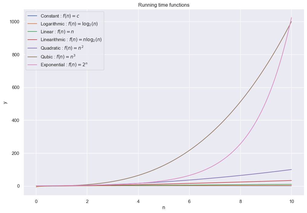
In running time analysis we analyse the number of operations an algorithms needs. Often we look at upper or lower bounds of the amount of operations.

running_times = {'Constant': lambda n : n**0,
                 'Logarithmic': lambda n : np.log2(n),
                 'Linear': lambda n : n,
                 'Linearithmic': lambda n : n * np.log2(n),
                 'Quadratic': lambda n : n ** 2,
                 'Qubic': lambda n : n ** 3,
                 'Exponential': lambda n : 2**n}
functions = [r'$f(n) = c$', r'$f(n) = \log_2(n)$', r'$f(n) = n$', r'$f(n) = n \log_2(n)$', r'$f(n) = n^2$', r'$f(n) = n^3$', r'$f(n) = 2^n$']

n = np.linspace(0.01, 10, 1000)

plt.figure(figsize=(12, 8))
plt.title('Running time functions')
for fl, fs in zip(running_times.keys(), functions):
    plt.plot(n, running_times[fl](n), label=f'{fl} : {fs}')
plt.xlabel('n')
plt.ylabel('y')
plt.legend()
plt.show();

Big O

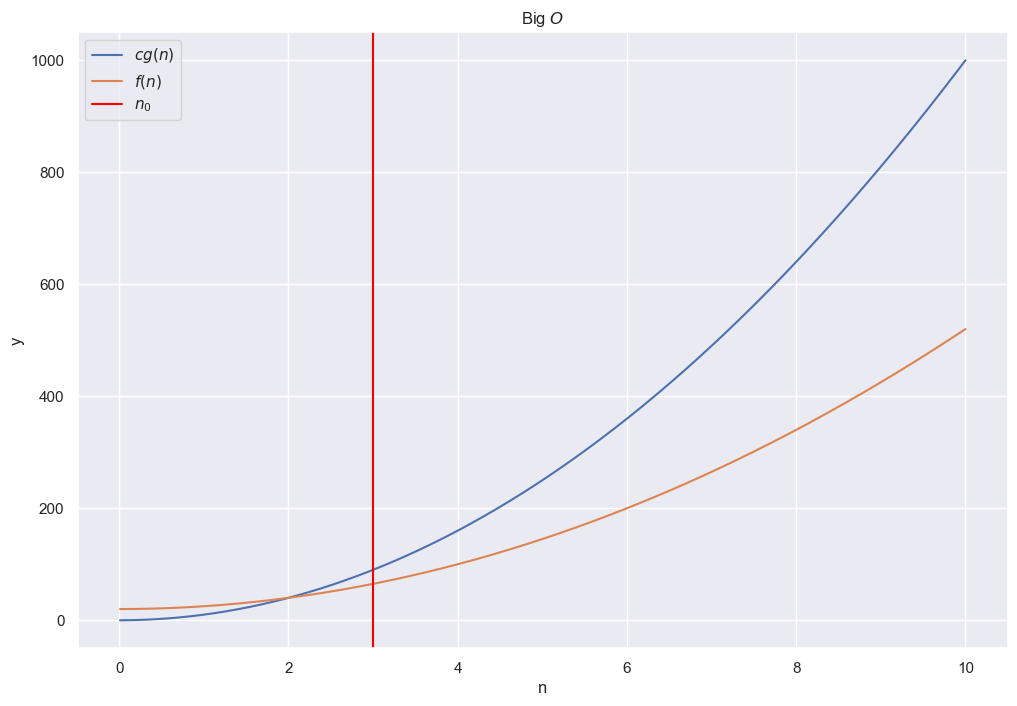
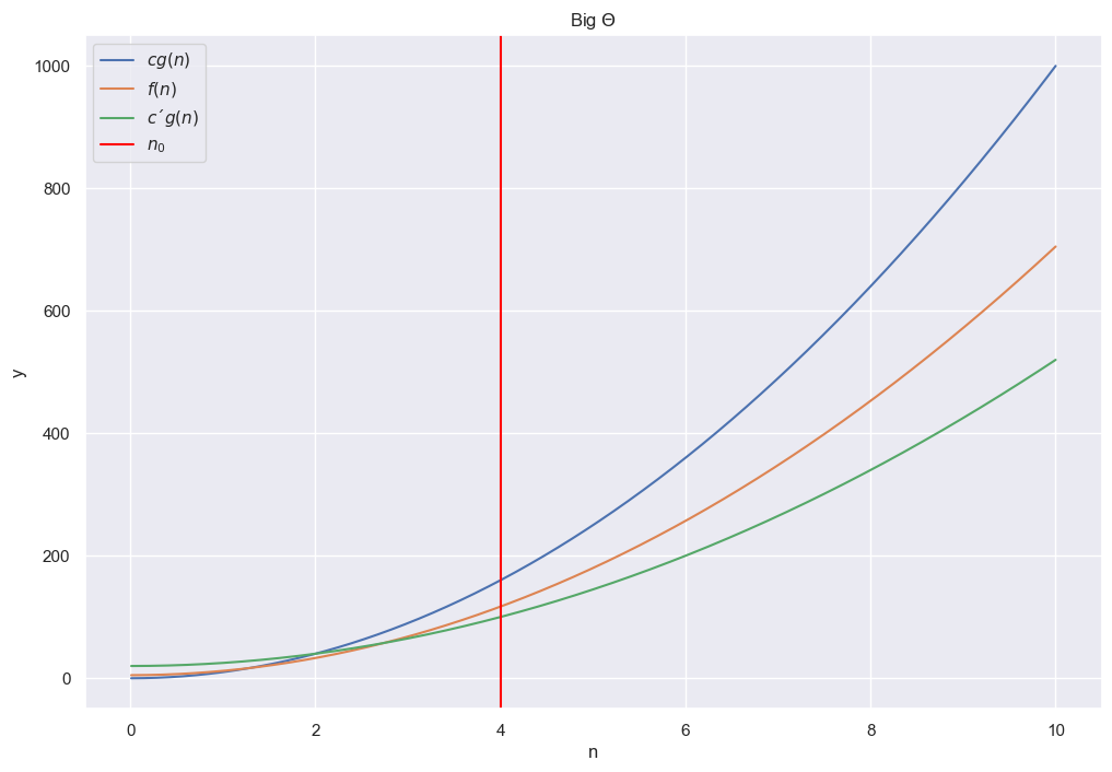
f1 = lambda n : 10 * n**2
f2 = lambda n : 5 * n**2 + 20

plt.figure(figsize=(12, 8))
plt.title(r'Big $O$')
plt.plot(n, f1(n), label=r'$cg(n)$')
plt.plot(n, f2(n), label=r'$f(n)$')
plt.axvline(x=3, label=r'$n_0$', color='red')
plt.legend()
plt.xlabel('n')
plt.ylabel('y')
plt.show();

Big $\Omega$

plt.figure(figsize=(12, 8))
plt.title(r'Big $\Omega$')
plt.plot(n, f1(n), label=r'$f(n)$')
plt.plot(n, f2(n), label=r'$cg(n)$')
plt.axvline(x=3, label=r'$n_0$', color='red')
plt.legend()
plt.xlabel('n')
plt.ylabel('y')
plt.show();

Big $\Theta$

f3 = lambda n : 7 * n**2 + 5

plt.figure(figsize=(12, 8))
plt.title(r'Big $\Theta$')
plt.plot(n, f1(n), label=r'$cg(n)$')
plt.plot(n, f3(n), label=r'$f(n)$')
plt.plot(n, f2(n), label=r'$c´g(n)$')
plt.axvline(x=4, label=r'$n_0$', color='red')
plt.legend()
plt.xlabel('n')
plt.ylabel('y')
plt.show();

Rules

1. $O(1) \subset O(\log_2 n) \subset O(n) \subset O(n \log_2 n) \subset O(n^2) \subset O(n^3) \subset O(2^n)$
2. If $f_1 \in O(g_1)$ and $f_2 \in O(g_2) \Rightarrow f_1 f_2 \in O(g_1 g_2)$
3. If $f_1 \in O(g_1)$ and $f_2 \in O(g_2) \Rightarrow f_1 + f_2 \in O(g_1 + g_2)$
4. If $f_1 \in O(g_1) \Leftrightarrow g_1 \in \Omega(f_1)$

Substitution method

For the substitution method we guess the form of our solution and show the correctness through the use of induction.

Consider the following recursion $T(m) = 2 T(m/2) + \Theta(m)$ with $m = 2^k$, $k \in \mathbb{N}_{> 0}$. Then by using substitution we get

Thus we guess that our running time is upper bounded by $O(m \log_2 m)$. Our hypothesis then becomes that our function is upper bounded $T(m) \leq c m \log_2 m$ for all $m\geq m_0$ for some $c, m_0 > 0$. We do the inductive step $m - 1 \rightarrow m$, where $m \geq 2 m_0$

Inductive steps works if we constrain c to be sufficiently large such that $cm \geq c′m$ for all $m \geq 2m_0$.

Now we need to show that $T(m) \leq cm\log_2 m$ for all $m$ with $m_0 \leq m \leq 2m_0$. Consider for this $m_0 = 2$.

Let $d = \max {T(2), T(3)}$. Then $T(2) \leq d \leq d 2 \log_2 2$ and $T(3) \leq d \leq d 3 \log_2 3$. With $c = \max{c’, d}$ it holds that for all $m \geq 2$ that

Recursion Tree Method

In the recursion tree method, each node represents the cost of a single subproblem in the recursive invocation. Analyzing the cost on each level of the tree and the depth of the tree gives an idea of the overall running time.

Master Theorem

The master theorem is often used for recurrent algorithms and is given by $T(n) = A T(n / B) + f(n)$. This is called the master recurrence, and the function $f(n)$ is called the driving function. The master theorem compares the asymptotic growth of the driving function to the one of the watershed function $n^{\log_B A}$.

Let $A \geq 1, B > 1$ be constant and $f(n)$ be a driving function that is defined and nonnegative on all sufficiently large reals. Let $T$ satisfy the master recurrence $T(n) = A T(n/B) + f(n)$. Then

Floor and Ceilings

Ignoring floors and ceilings does not generally affect the order of growth of the solution of a divide-and-conquer recurrence.