Parameter Estimation

import numpy as np
import matplotlib.pyplot as plt

Taxi cab problem

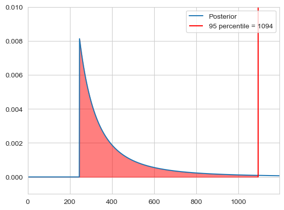
Imagine we observe $c$ taxi cabs, with $m$ being the largest one. We set our hypothisis as $\mathcal{H}_n$ that there are in total $n$ taxis. We use a uniform prior $\mathbb{P}(\mathcal{H_n} | I) = \text{constant}$ and define our likelihood as $\mathbb{P}(\mathcal{D} | \mathcal{H_n} I) = \frac{\theta(n - m)}{n \cdot (n - 1) \cdot … \cdot (n - c + 1)}$, where $\theta(x)$ is zero when $x < 0$ and 1 if $x \geq 0$. We can then calculate the probability of how many taxis there are in total, which is given by the posterior:

Here we just set k to 1000 as an upper limit. Then we can calculate our $n$ for a certain confidence, for example 95%:

data = [33, 125, 246]
upper = 1000000
n = np.arange(0, upper + 1, 1)

likelihood = []
for i in n:
    if (i - max(data)) >= 0:
        likelihood.append(np.exp(-np.log(i) - np.log(i - 1) - np.log(i - 2)))
    else:
        likelihood.append(0)    

evidence = np.sum(likelihood)
posterior = likelihood / evidence

n_95 = np.argmax(np.cumsum(posterior) > 0.95)

plt.plot(n, posterior, label='Posterior')
plt.fill_between(n[:n_95], posterior[:n_95], alpha=0.5, color='red')
plt.vlines(n_95, ymin=0, ymax=0.5, color='red', label=f'95 percentile = {n_95}')
plt.legend()
plt.ylim([-0.001, 0.01])
plt.xlim([0, n_95 + 100])
plt.show()

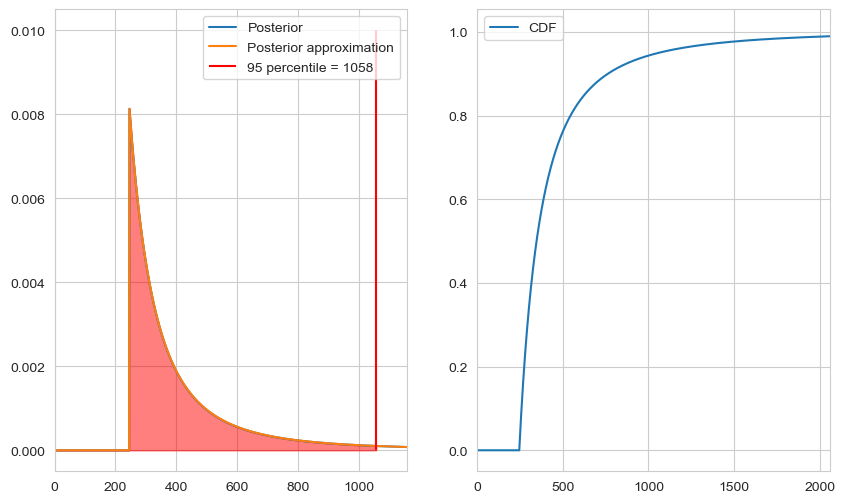
For large $m$ we can again approximate the factorial by the power $\frac{1}{n \cdot(n - 1) \cdot … \cdot (n - c + 1)} \approx \frac{1}{n^c}$ and calculate our normalisation constant as

Thus we get the distribution

data = [33, 125, 246]
upper = 1000000
n = np.arange(0, upper + 1, 1)

c = len(data)
m = max(data)

posterior_approx = []
for i in n:
    if i >= m:
        posterior_approx.append(((c - 1) / m) * (i / m)**(-c)) 
    else:
        posterior_approx.append(0)

n_95 = np.argmax(np.cumsum(posterior_approx) > 0.95)

fig, axs = plt.subplots(1, 2, figsize=(10, 6))

axs[0].plot(n, posterior, label='Posterior')
axs[0].plot(n, posterior_approx, label='Posterior approximation')
axs[0].fill_between(n[:n_95], posterior[:n_95], alpha=0.5, color='red')
axs[0].vlines(n_95, ymin=0, ymax=0.01, color='red', label=f'95 percentile = {n_95}')
axs[0].legend()
axs[0].set_xlim([0, n_95 + 100])

axs[1].plot(n, np.cumsum(posterior_approx), label='CDF')
axs[1].set_xlim([0, n_95 + 1000])
axs[1].legend()

plt.show()

Features of this distribution are:

Mode is always at $n = m$

We can find our $\alpha$ % intervall by calculating the probablity:

Which then gives us our intervall $[m, m \epsilon^{-1/(c-1)}]$.

The mean is given by

The median is given by

But the question that remains is, which is the best function to describe our $n$?

We define the loss function $L(r, n)$ which gives us a cost (penalty) for predicting a value $r$ if the the true value is $n$. Then logically we want to minimize our penalty for guessing a value $r$, so we pick $r$ which minimizes our loss function.

Linear loss

The linear loss function is given by $L(r, n) = |r - n|$. To then minimize this function, we know that $\langle L(r) \rangle$ is a strict convex function, which has a definit minima so we take it’s derivate and set it to zero

Quadratic loss

The quadratic loss function is given by $L(r, n) = (r - n)^2$. Same rules apply and we get:

Delta loss

The delta loss function is given by $L(r, n) = 1 - \delta(r, n)$, where $\delta(r, n)$ is 0 for r = n and 1 everywhere else.

This function clearly takes it’s minima at the value of $r$ which has the highest probability, which is the mode $r = n_*$

Probability density

Let $p$ be a probability, then $\mathbb{P}(p | \mathcal{D}, I)dp$ is the probability that $p$ lies in between $p$ and $p + dp$. If we then want to find the probability that $p$ is in a given intervall, for continous problems we can calculate this by an integral

Beta distribution

we get the posterior for our probability p given the data as:

This is called the beta distribution. The general form of the beta distribution is:

With $B(\alpha, \beta) = \int_0^1 p^{\alpha - 1} (1 - p)^{\beta - 1} = \frac{\Gamma(\alpha)\Gamma(\beta)}{\Gamma(\alpha + \beta)}$

The beta distribution has the following properties

It’s mode is given by $p_* = \frac{\alpha - 1}{\alpha + \beta - 2}$

It’s mean is given by $\langle p \rangle = \frac{\alpha}{\alpha + \beta}$

The variance is given by $\langle p^2 \rangle - \langle p \rangle^2 = \frac{\langle p \rangle (1 - \langle p \rangle)}{\alpha + \beta + 1}$

Transforming probability densities

Imagine we have a virus which kills cells at a constant rate per unit time $p(\text{die in time dt}) = \lambda dt$, if f(t) is the fraction of cells that are alive after time t we get

Assume we collect $m$ infected cells and determine that $k$ of $m$ cells are still alive. With this we can estimate the total fraction of cells $p$ that is still alive. This is given by the beta distribution. But what if we’re interested in the time $t$ at which the cells were infected? We then would like to be able to transform our posterior on the probability $\mathbb{P}(p, | m, k)dp$ into a posterior on the infection time $\tilde{\mathbb{P}}(t | m, k) dt$.

Given the function $t(p) = - \frac{\ln(p)}{\lambda}$, we know that the probability for $p$ to lie in a specific region is the same as for $t$ to lie in the corresponding region

Which is equivalent to the substitution $t(p) = - \frac{\ln (p)}{\lambda} \Rightarrow dt = - \frac{1}{p \lambda} dp$: \(\int_{p_{min}}^{p_{max}} \mathbb{P}(p | m, k) dp = - \int_{t(p_{max})}^{t(p_{min})} \tilde{\mathbb{P}}(t(f) | m, k) \frac{dt}{df} df = \int_{t(p_{min})}^{t(p_{max})} \frac{1}{\lambda p} \tilde{\mathbb{P}}(t(f) | m, k) dt\)

From which follows then the rule of transformation:

Here then we get the specific distribution