Quantitation Probabilities
For looking at probability of events, we set the following defintions. Let $A$ be an event and $I$ the given information: $\mathbb{P}(A | I)$: The probab...
import numpy as np
from scipy.special import gammaln
from matplotlib import pyplot as plt
import seaborn as sns
import scipy as sp
sns.set_theme()
Imagine we have a box with a total of $T$ balls in it, where among these, we have a total of $r$ red balls. If we now take out $n$ balls, how many of these are red? We can imagine this as that each ball has a number from $1$ to $T$ and we take out a ball one by one. Then for the first ball, we have a total of $T$ possible balls from which we can pick, the second time we only have $T - 1$ balls left etc. With this we get:
\[T \cdot (T - 1) \cdot (T - 2) \cdot ... \cdot 2 \cdot 1 = T!\]Which is the total amount of arrangements of our numbered $T$ balls. Then taking only $n$ balls from $T$ gives us:
\[T \cdot (T - 1) \cdot (T - 2) \cdot ... \cdot (T - n) = \frac{T!}{(T - n)!}\]From our first $n$ picked balls, these have $n!$ combinations we do not care about, so we divide by these amount of combinations to get out total amount of possibilities of taking $n$ balls out of $T$:
\[N = \frac{T!}{n!(T - n)!} = \begin{pmatrix} T \\ n \end{pmatrix}\]This is the so called binomial coefficient. Because we then have no means of differentiating between these differnt possibilities, we get the uniform probability $\mathbb{P}(A_i | I) = \frac{1}{N}$ for all these possibilities, because there are $N$ different subsets when picking $n$ from $T$. If we now want to find out the probability of having $k$ red balls in our $n$ balls, we’d have to sum over all possibilities in $N$ where we have $k$ red balls:
\[\mathbb{P}(k | I) = \frac{N(k)}{N}\]Looking at our $n$ picked balls, the amount of possibilities of having $n - k$ blue balls is given by $\begin{pmatrix} T - r \ n - k \end{pmatrix}$ and the possibilities of having k red balls are $\begin{pmatrix} r \ k \end{pmatrix}$ Thus in total we get
\[N(k) = \begin{pmatrix} T - r \\ n - k \end{pmatrix} \begin{pmatrix} r \\ k \end{pmatrix}\]The probability of then having k red balls out of our sample of size $n$ from the total amount of balls $T$ is given by the so called hypergeomtric distribution:
\[\mathbb{P}(k | I) = \frac{\begin{pmatrix} T - r \\ n - k \end{pmatrix} \begin{pmatrix} r \\ k \end{pmatrix}}{\begin{pmatrix} T \\ n \end{pmatrix}}\]For large $T$ and smallr $n$ and $k$ we can approximate the factorial by a power multiplication, $(T - n)! \approx T^n$. By using this approximation we can transform our hypergeometric distribution into the so called Binomial distribution:
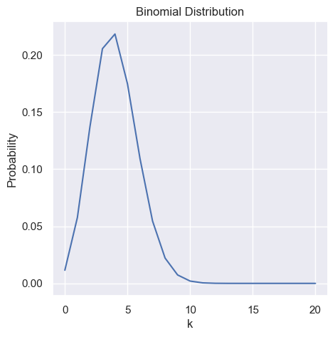
\[\mathbb{P}(k | I) = \begin{pmatrix} n \\ k \end{pmatrix} \left( \frac{r}{T} \right)^k \left(1 - \frac{r}{T} \right)^{n - k}\]
p = 0.2
n = 20
k = np.arange(0, n + 1, 1)

binomial = sp.stats.binom(n, p)
prob = binomial.pmf(k)

plt.figure(figsize=(5, 5))
plt.plot(k, prob)
plt.xlabel('k')
plt.ylabel('Probability')
plt.title('Binomial Distribution')
plt.show()
Given a distribution $\mathbb{P}(k | I)$ the mean, average or expected value of this distribution is given as:
\[\langle k \rangle = \sum_k k \mathbb{P}(k |n, p)\]For a fixed set, the mean is given as $\bar{k} = \frac{1}{n} \sum_{i = 1}^n k_i$
The mean of the binomial distribution is given as $\langle k \rangle = np$
The mode of a distribution is the most likely value, the value that most often appears in a given dataset of the distribution.
Let $k_*$ be the value of $k$ with the highest probability, the mode is given by
\[(n + 1)p - 1 < k_* < (n + 1)p\]and for large $n$ this converges to the expected value $np$.
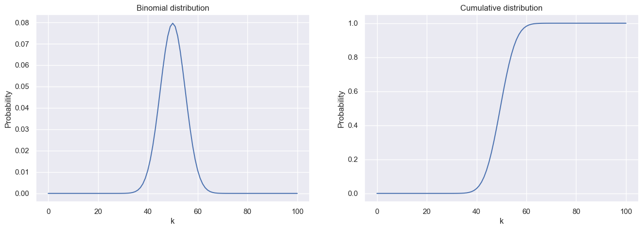
We may, instead of wanting the probability of a specific $k$, the probability of a value being less or equal $k$: $\mathbb{P}(x \leq k |n, p)$. This is the so called cumulative function and can be written as:
\[C(k | n, p) = \sum_{i = 0}^k \mathbb{P}(i | n, p)\]n = 100
k = np.arange(0, n + 1, 1)
p = 0.5
binomial = sp.stats.binom(n, p)
prob = binomial.pmf(k)
fix, axs = plt.subplots(1, 2, figsize=(16, 5))
axs[0].plot(k, prob)
axs[0].set_title('Binomial distribution')
axs[0].set_xlabel('k')
axs[0].set_ylabel('Probability')
axs[1].plot(k, np.cumsum(prob))
axs[1].set_title('Cumulative distribution')
axs[1].set_xlabel('k')
axs[1].set_ylabel('Probability')
plt.show()
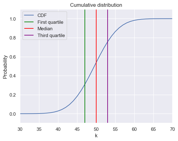
Quantiles are used to indicate how many values are above or below a certain limit.
n = 100
k = np.arange(0, n + 1, 1)

binomial = sp.stats.binom(n, p)
prob = binomial.pmf(k)
c = np.cumsum(prob)

plt.plot(k, c ,label='CDF')
plt.title('Cumulative distribution')
plt.xlabel('k')
plt.ylabel('Probability')

plt.vlines(x=np.argmax(c > 0.25), ymin=-2, ymax=2, color='green', label='First quartile')
plt.vlines(x=np.argmax(c > 0.5), ymin=-2, ymax=2, color='red', label='Median')
plt.vlines(x=np.argmax(c > 0.75), ymin=-2, ymax=2, color='purple', label='Third quartile')

plt.ylim([-0.1, 1.1])
plt.xlim([30, 70])
plt.legend()
plt.show()
The variance is defined as the expected square deviation from the mean
\[var(k) = \langle (k - \langle k \rangle)^2 \rangle = \langle k^2 \rangle - \langle k \rangle ^2 = \sum_k (k - \langle k \rangle )^2 \mathbb{P}(k)\]The standard deviation is then just the square root of the varianve: $std(k) = \sqrt{var(k)}$
The variance of the binomial distribution is given as
\[var(k) = np(1 - p)\]Looking at the inverse problem, where we don’t know the probability $p$ but we know our sample size $n$ and how many times we observe a certain event as $k$, how can we go from our probability $\mathbb{P}(k | p, n)$ to the probability $\mathbb{P}(p, | k, n)$. Which is to say, how can we go from our observation to the distribution of the underlying probability given our data.
Within the prior we can encode our information we already know of our distribution, like it’s size. We denote $\mathcal{H}_n$ as our prior hypothisis, where $n$ is the size of our problem. These hypothisis are exhaustive and mutually exclusive (M.E.E). Incase of no real prior information, we just use an uniform prior.
With the likelihood, we calculate the probability of observing our data. Let $\mathcal{D}$ be our data, then we can write our likelihood as:
\[\begin{align*} \mathbb{P}(\mathcal{D} | I) &\overset{M.E.E}{=} \mathbb{P}(\mathcal{D} \sum_n \mathcal{H}_n | I) \\ &= \mathbb{P}(\sum_n \mathcal{D} \mathcal{H}_n | I) \\ &\overset{M.E.E}{=} \sum_n \mathbb{P}(\mathcal{D} \mathcal{H}_n | I) \\ &\overset{\text{Product rule}}{=} \sum_n \mathbb{P}(\mathcal{D} | \mathcal{H}_n I) \mathbb{P}(\mathcal{H}_n | I) \end{align*}\]Here $\mathbb{P}(\mathcal{H}_n | I)$ denotes the probability of our hypothisis for size $n$ being true and $\mathbb{P}(\mathcal{D} | \mathcal{H}_n I)$ denotes the probability of observing our data given the hypothisis of size $n$ and our information $I$. The summation over all $n$ gives then the total probability of our data.
With the given prior and likelihood we can calculate our wanted calculation by the use of the product rules. The bayes theorem is given by:
\[\mathbb{P}(\mathcal{H}_n | \mathcal{D} I) = \frac{\mathbb{P}(\mathcal{D}| \mathcal{H}_n I)\mathbb{P}(\mathcal{H}_n | I)}{\mathbb{P}(\mathcal{D}| I)} = \frac{\mathbb{P}(\mathcal{D}| \mathcal{H}_n I)\mathbb{P}(\mathcal{H}_n | I)}{\sum_i \mathbb{P}(\mathcal{D} | \mathcal{H}_i I) \mathbb{P}(\mathcal{H}_i | I)}\]The probability $\mathbb{P}(\mathcal{H}_n | \mathcal{D} I)$ is the so called posterior. The bayes formula can be thought of as the updating of our prior belief after observing the data, the posterior gives then the probability of how likely the data is given the specific hypothisis over how likely it is in general to get this data.
For looking at probability of events, we set the following defintions. Let $A$ be an event and $I$ the given information: $\mathbb{P}(A | I)$: The probab...
import numpy as np from scipy.special import gammaln from matplotlib import pyplot as plt import seaborn as sns import scipy as sp sns.set_theme()
import numpy as np import matplotlib.pyplot as plt
import scipy as sp import numpy as np import matplotlib.pyplot as plt
import scipy as sp import numpy as np import matplotlib.pyplot as plt
Difference trial and reference sample
Linear Regression discrepancy
```python import numpy as np import matplotlib.pyplot as plt from scipy.special import gamma import seaborn as sns
import numpy as np import matplotlib.pyplot as plt import seaborn as sns from matplotlib import cm sns.set_theme()